As long as their amplitudes are small, two waves in the same physical location do not interact with each other. This implies that when two or more waves are superimposed on each other, the net wave displacement is just the algebraic sum of the displacements of the individual waves. Since these displacements can be positive or negative, the net displacement can either be greater or smaller than the individual wave displacements. The former case is called constructive interference, while the latter is called destructive interference. Interference between the same two waves can be constructive at a given point of space and destructive at another point, depending on their phase relation at the two points (see figure 1). Therefore the signal's amplitude varies as a function of the position in space, displaying a chessboard-like pattern that is the signature of interference.
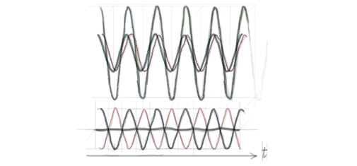
Figure 1. The green wave results from the superposition of the blue and red waves at a point O (waves are here represented as a function of time). If the blue and red waves oscillate in phase ('crests' superposed), the interference is constructive and the signal in O is enhanced (top); if they oscillate in opposition (blue 'throughs' superposed to red 'crests'), the interference is destructive and no signal is observed in O (bottom).
To compare the behavior of particles and waves we shall analyse a double-slit interferometer. The design of the set-up, which is based on an experiment carried out by Thomas Young more than two hundred years ago, is showed in figure 3. Suppose first that we have a gun shooting a stream of bullets. The bullets have to pass through a filter with two vertical slits in order to impinge on the detection plate. Figure 5 shows the distribuition of detected bullets as a funtion of the longitude x on the detection plate, for different arrangements. (Because of the symmetries of the problem, x is the only relevant coordinate.) The red curve refers to a set-up in which only slit 1 is open while slit 2 is blocked. The blue curve refers instead to a set-up in which slit 2 is open and slit 1 is blocked. The Green curve A is the distribution observed when both slits are open. As one expects based on elementary statistics, the green curve A is just the (weighted) sum of the blue and the red ones.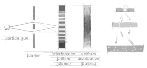
Figure 2. Double slit experiment with bullets. No interference pattern is observed.
We now repeat the same experiment after replacing the gun with a source of monochromatic light. Instead of the number of bullets, we measure the light intensity. Assuming that the relevant parameters are properly adjusted, the intensity distribution when the two slits are open displays interference fringes, i.e. alternate maxima and minima. Unlike in the bullets experiment, here the total intensity distribution (green curve B) cannot be regarded as the algebraic sum of the independent contributions coming from each slit (red and blue curves). This result can be easily understood taking into account the wavelike nature of light and admitting that the wave emitted by the source is split into two secondary waves. Depending on their phase relation at each point of the detection plate, the two waves add up constructively or destructively, giving rise to alternate maxima and minima in the measured intensity. Figures 2 and 3 show the typical behaviors of classical particles (bullets) and classical waves in a double-slit experiment.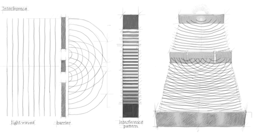
Figure 3. Double slit experiment with waves. The two slits create a phase difference that make the two waves interfere with each other. Bright fringes are observed at places where the interference is constructive, darks fringes where the interference is destructive.
Now we come to atoms. If the same kind of experiment is performed using an atom beam, the result is not the one we get with bullets; rather, the distribution of the atoms detected at the detection plate displays interference fringes, as in the case of light (figure 3)!One might conclude that this must be because atoms really are waves. The problem with this conclusion is that, regardless of the detection technique employed, we always detect individual, well-localized spots, just as in the case of bullets. In fact, only when an ensemble of atoms has been recorded, interference fringes become apparent: ‘bright’ fringes where a lot of individual atoms impinged and ‘dark’ fringes where no atoms were recorded (see figure 6). The whole process looks as if the statistical behavior of the atoms were ruled by some wavelike law (see origins).
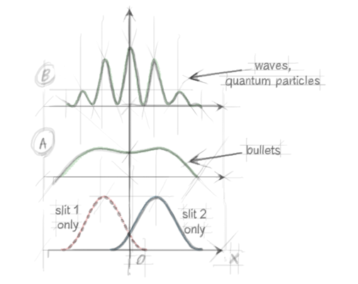
Figure 4. The four curves represent the probability of detecting one particle at point x. The red (blue) distribution is observed both with particles and waves when only slit 1(2) is left open while slit 2(1) is blocked (see Uncertainty). Green distribution A is observed with classical particles when both slits are open. Interference fringes B are observed with quantum particles and waves when both slits are open.
It is worth considering one more variant of the experiment. Let's suppose that our atoms are excited . This means that they are likely to decay to a lower energy level emitting a photon. Assume further that the photon is very likely to be emitted exactly while the atom is passing through the filter. In principle, the apparatus could be equipped with photon detectors allowing one to tell which slit the emitted photon comes from. This means that the very fact of using excited atoms puts one in a position to distinguish (at least in principle) which slit the atom passed through. Notice that this piece of information is essentially incompatible with the model that associates two secondary waves (one for each slit) with each atom. Surprisingly enough, when an ensemble of atoms is recorded under these experimental conditions, interference fringes are not observed, and the uniform distribution observed with bullets (figure 4A) is recovered. This happens even though the photon is not detected. Assume further that the photon detector is not actually in place. We get the impression that the possibility of monitoring the atoms' path forces them to behave like classical particles (see origins for further discussion).
Figure 5. The interference pattern disappears if a piece of information correlated with the particle's path is disseminated in the environment.
Historically, the corpuscular nature of light became apparent before the implementation of diffraction experiments with particles. In the early 20th century, the discovery of the photoelectric effect and of the Compton effect showed that, under some circumstances, photons and electrons scatter each other like billiard balls do. Nowadays, single photons can be stored in superconducting cavities and manipulated by means of individual atoms, emphasizing at will either the wavelike or the corpuscular nature of light.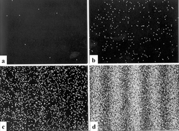